In a previous post I created a guitar model classifier that was capable of discriminating between two iconic guitars (the Gibson Les Paul and the Fender Stratocaster). Using a ResNet-34 architecture and the fastai v0.7 deep learning python package I created a model that could predict the right class with 95.4% accuracy.
In a next step I wanted to expand this to a multi-class classification. Since then, a new version of fastai launched that builds on the pre-release of pytorch 1.0 and features a pretty different architecture but many substantial improvements. The following results are based on version 1.0.26 (but please check for updates, the library is currently evolving basically on a daily basis).
Fast.ai v1 quick intro
One of the greatest improvements in version 1.0 is a proper documentation page. Due to the rapid development it too changes basically daily, but most foundational APIs seem to be in place now. One noteworthy thing is that the documentation is build from Jupyter notebooks and thus all code can be run from the doc_src directory at their GitHub repository. As mentioned, fastai v1 consists of four applications: vision (image classification, segmentation, etc.), text (natural language processing), tabular (structured data), and collab (collaborative filtering) [see Figure 1]. Apart from collab, all applications are structured into transformations (data pre-processing, data augmentation, tokenization, etc.), data (dataset classes for the specific use case), models (actual model architectures). Data and models are combined into a learner.
One big change occurred at version 1.0.22 (I think, things move fast) when the data block API was introduced. I will use this API in this post instead of the older dedicated vision tools as it’s a more generic option and translates nicely also into the other fastai components tabular, text, and collab. In general, you specify the following components that together are used to create a DataBunch - the container that holds training, validation and test data as well as information about data augmentation.
Building a dataset with fastclass
Before we start we need a dataset of images. You can use one of the provided datasets, get your data from kaggle, google, or build your own. I recently wrote the small toolkit fastclass to make the process of downloading and cleaning a custom dataset easier (see blog post and GitHub repo).
Note: I provide the full jupyter notebook here. The dataset can be downloaded from within the notebook off a dropbox link. The guitar dataset consists of approx. 8500 images from 11 different guitar classes (five Fender models and six Gibsons).
Starting: ResNet-34
Using the new data block API we build a DataBunch from the images in our dataset. Since we reuse this bit of code later I divided it into two parts (training and validation data split; image transformation):
# Since src will be reused later and we need to have the same
# images in train and validation sets to avoid data leakage
src = (ImageItemList.from_folder(pathlib.Path.cwd()/'data/guitars')
           .random_split_by_pct()
           .label_from_folder(classes=classes))

# Return a DataBunch with specified image and batch
# size
def get_data(src, sz=224, bs=64):
    """get new databunch with requested resolution"""
    return (src.transform(get_transforms(do_flip=False), size=sz)
               .databunch(bs=bs)).normalize(imagenet_stats)

# example: get a databunch with images of size 299x299 and
#          a batch size of 32
data = get_data(src, sz=299, bs=32)
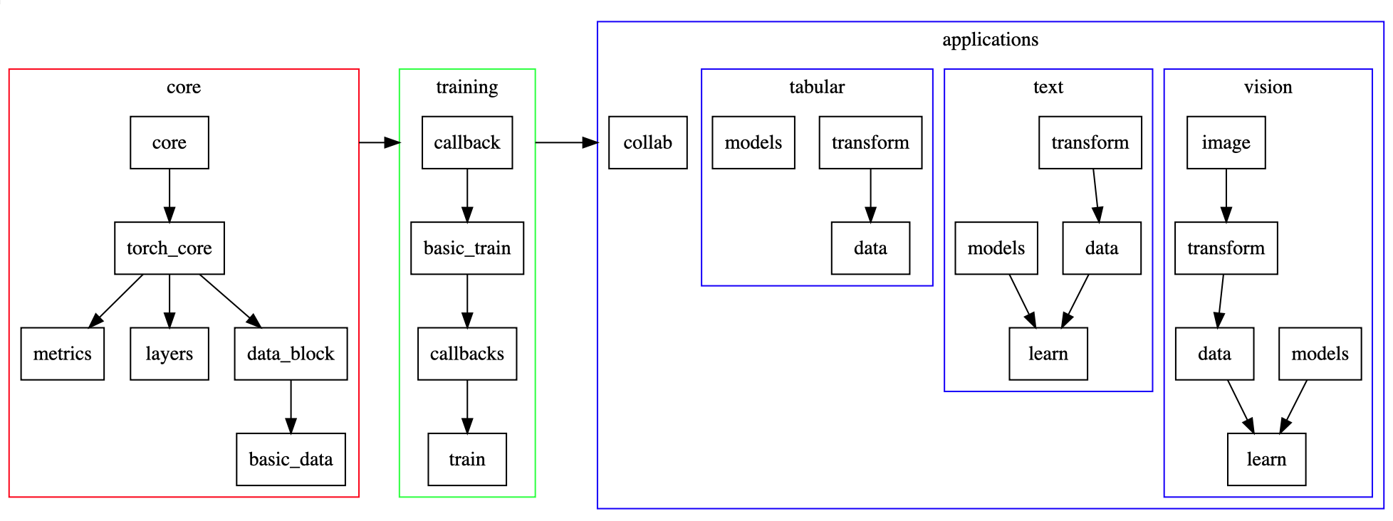
To have a quick look we can display a sample of the data with:
data.show_batch(rows=3, figsize=(8,6))
To get started we do not train a model from scratch as a model pretrained on a large image dataset is always preferable to learning from random weight initializations. Using transfer learning we can leverage the substantial compute efforts that went into an existing model (ResNet-34 in this case, trained on > 1 million ImageNet images). We will reuse this knowledge and replace the head of the model with a new set of fully-connected layers dedicated to our classification task.
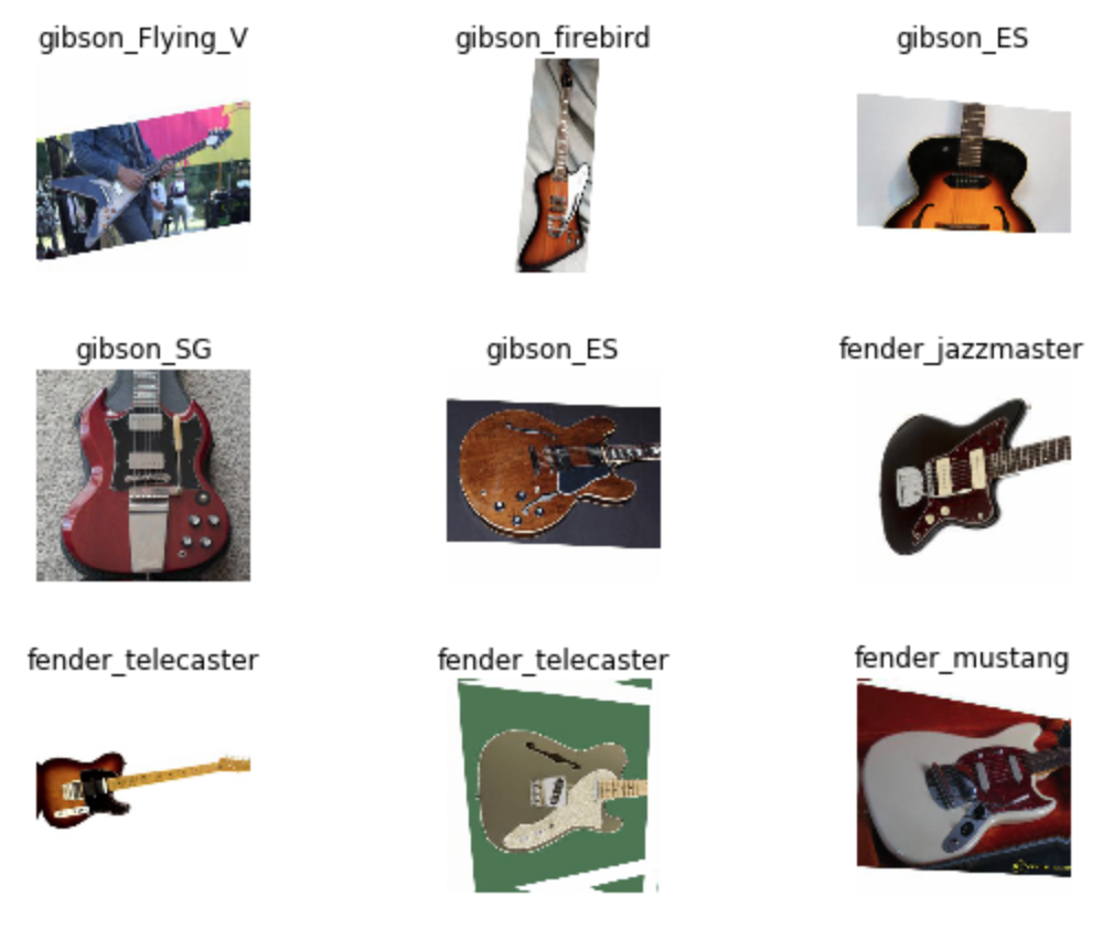
We start with the ResNet-34 base model and a DataBunch containing images of size 224x224 (bs=64). To track our progress we specify the error_rate as a metric. First, we run the learning rate finder to determine the optimal learning rate to improve our model quickly.
learn = create_cnn(data, models.resnet34, path='.', metrics=error_rate)
learn.lr_find();
learn.recorder.plot()
As is clear from the plot, we want to find a learning rate that gives us the smallest loss rate while making the biggest steps in the feature space. As a rule of thump we thus find the lowest point on the curve before the loss shoots up again and go one magnitude to the left (0.01 in this case). We then train the model for five cycles using the fit_one_cycle() method. The one cycle policy is a great technique of setting the hyper parameters (learning rate, momentum and weight decay) in a way to train complex models fast and efficient (it’s the standard approach in fastai). In essence, we want the biggest possible learning rate (determined by lr_find()) to explore the feature space efficiently. Second, the learning rate changes in a cycle from a low value (10 times lower than the lf_find() result) up to the maximum and then back down again. It was observed that the high learning rates at the middle of a cycle also act as regularization method that prevents overfitting. In addition, the momentum of the stochastic gradient descent (SGD) is altered in an anti-cyclical pattern.
lr = 0.01
learn.fit_one_cycle(5, slice(lr))
After only 4:34 min on a K80 GPU we already have a model capable of predicting the right guitar model from a set of eleven classes with 95.1% accuracy!
Total time: 04:34
epoch  train_loss  valid_loss  error_rate
1      0.928203    0.450700    0.162353    (00:57)
2      0.536406    0.311858    0.098824    (00:54)
3      0.347128    0.200679    0.065882    (00:54)
4      0.225095    0.175412    0.053529    (00:54)
5      0.162299    0.157303    0.049412    (00:54)
We save the model and proceed to improve it by fine-tuning also the lower layers in the architecture (up till now we only trained the new head of the model). First, we unfreeze the model (now all weights will be trained) and run the learning rate finder again to determine the optimal learning rate.
learn.load('guitars-v1-11cl-res34-224px-01')
learn.unfreeze()
learn.lr_find()
learn.recorder.plot()
We set the learning rate to 1e-05 for the lower layers of the model and 0.005 for the head (this is called a discriminate learning rate) as we do not want to destroy to learned features in the lowest layers. Those detect simple features (edges, gradients, simple patterns) that should be pretty universal for all kinds of images. We got them from the pertained model for free and they are based on the model learning from millions of images. After five more cycles (another 6:20min of training) we end up with a model that can predict with 97.3% accuracy.
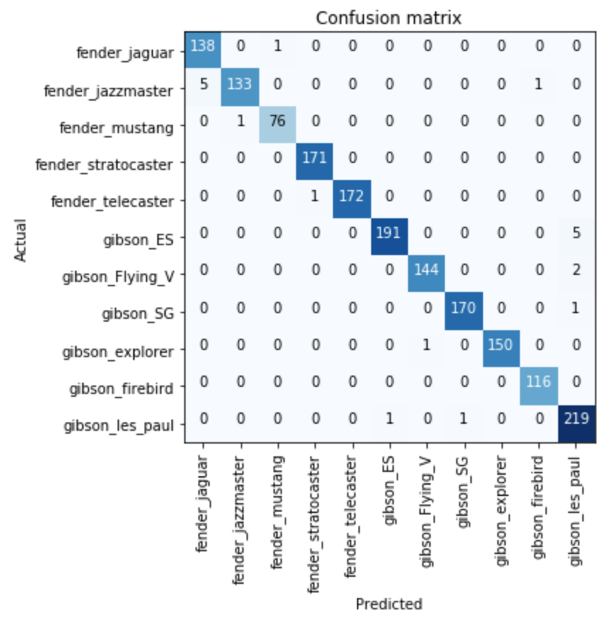
When we inspect the confusion matrix of the model, we can see where the model get’s it wrong.
# plot a confusion matrix
interp = ClassificationInterpretation.from_learner(learn)
interp.plot_confusion_matrix(figsize=(8,6))

# show largest classification errors
display(interp.most_confused(min_val=2))

Seems the model has a hard time differentiating between a Fender Jaguar and Jazzmaster (who wouldn’t - they are super similar). Dito for the Gibson ES and Les Paul (here, special models exist that lend features from the other guitar ranges, i.e. f-holes, pickup configurations, …).
Level up: ResNet-50
While this result is already quite impressive, we so far only used a relative simple model architecture. We now progress to ResNet-50, that features substantially more layers and thus weights that can potentially learn more features of our data. To not exceed our GPU memory we have to reduce the batch size now from 64 to 32.
First, we build a new DataBunch with the same train/ validation split but the smaller bs=32. We then create a new model based on the ResNet-50 architecture and run our learning rate finder again (the optimum learning rate seems to be 0.01). We immediately train the model for five cycles.
data = get_data(src, sz=224, bs=32)

learn = create_cnn(data, models.resnet50, path='.', metrics=error_rate)
learn.freeze()
learn.lr_find();
learn.recorder.plot()

lr = 0.01
learn.fit_one_cycle(5, slice(lr))
Then, we again train the entire model architecture with discriminative learning rates:
learn.load('guitars-v1-11cl-res50-224px-01')
learn.unfreeze()
learn.lr_find()
learn.recorder.plot()

learn.fit_one_cycle(5, slice(1e-6, lr/5))
learn.save('guitars-v1-11cl-res50-224px-02')
After these 2x5 cycles we now have an accuracy of 98%.
Total time: 10:28
epoch  train_loss  valid_loss  error_rate
1      0.591651    0.319690    0.105294    (02:11)
2      0.461109    0.398586    0.115294    (02:04)
3      0.292784    0.192599    0.067647    (02:04)
4      0.178708    0.128503    0.041176    (02:04)
5      0.098652    0.102441    0.033529    (02:03)

Total time: 13:47
epoch  train_loss  valid_loss  error_rate
1      0.122527    0.123221    0.032353    (02:46)
2      0.131352    0.129197    0.040588    (02:45)
3      0.084470    0.085018    0.028235    (02:45)
4      0.055003    0.071305    0.022353    (02:45)
5      0.035648    0.065091    0.020000    (02:45)
Progressive resizing
In order to improve the model even more, we now use a technique called progressive resizing. We feed the model larger versions of our images (448x448px instead of the previous 224x224) and again reduce our batch size (bs=16).
# load the previous model version from storage
learn.load('guitars-v1-11cl-res50-224px-02')

# feed the new data (448x448px)
learn.data = get_data(src, sz=448, bs=16)
learn.freeze()
The learning rate finder tells us to use a maximum learning rate of 0.001 and thus we train the head of the model for five cycles.
Lr = 0.001
learn.fit_one_cycle(5, slice(lr))
learn.save('guitars-v1-11cl-res50-448px-01')
With the bigger architecture and substantially larger images we now have to wait for 38 minutes.
Total time: 37:46
epoch  train_loss  valid_loss  error_rate
1      0.183134    0.086426    0.028235    (07:42)
2      0.099537    0.067973    0.020588    (07:30)
3      0.091131    0.060259    0.015294    (07:31)
4      0.062417    0.050117    0.013529    (07:30)
5      0.049533    0.048065    0.013529    (07:31)
However, as you can see the accuracy of the model improved drastically! Compared to the previous model, we now have an accuracy of 98.6% (a relative error rate improvement of 30%!). Again, we also train the full model.
learn.load('guitars-v1-11cl-res50-448px-01')
learn.unfreeze()
learn.fit_one_cycle(5, slice(1e-06, lr/5))
This takes even longer (49:50min):
Total time: 49:52
epoch  train_loss  valid_loss  error_rate
1      0.067349    0.044458    0.015294    (10:02)
2      0.055378    0.056939    0.015294    (09:57)
3      0.050544    0.045030    0.011765    (09:57)
4      0.034476    0.040948    0.012353    (09:57)
5      0.032105    0.041326    0.011765    (09:57)
We improve the accuracy again: the final model now has an accuracy of 98.8%. If we check the confusion matrix we see that almost all validation files are predicted correctly.
Conclusion
As shown, it takes relative little effort to build a custom image classifier capable of some extremely high accuracy. Using a deep learning library like fastai, a pre-trained model architecture, a reasonably-size dataset and some tricks can get you a long way!
What’s next
In the next blog posts I will look at Class Activation Maps to see which regions of an image actually ‘trigger’ the classification. Furthermore, I want to write a small post about how to deploy the model with a flask web app. So stay tuned.
The notebook can be found here.