
As part of the Coursera course Communicating Data Science Results I want to present my assignment in this blog post. The aim of the assignment is to analyze and visualize crime incident data for the cities Seattle and San Francisco.
Note: Instead of the provided small subset (summer 2014) of crime data I used a full year worth of data from the original data sources (year: 2017):
The actual jupyter notebooks are located at my github
Report
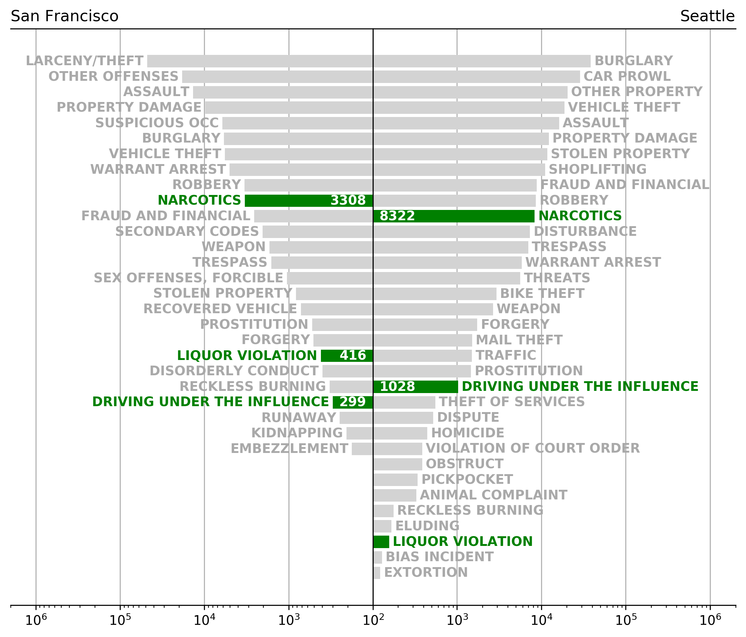
The following analysis reports on alcohol and narcotic related offenses as reported by the San Francisco and Seattle police departments for the year 2017. The most common offenses reported for San Francisco are “Larceny/Theft”, “Other offences”, “Assault”, whereas the Top 3 for Seattle are “Burglary”, “Car Prowl”, “Other Property”. However, it has to be noted that both data schema are not fully compatible and thus a class mismatch is likely (also, the summary classes are not disentangled). For the preprocessing carried out prior to this analysis and the individual code that produced these plots please see the jupyter notebook here rank on position 10, 20, and 23 (San Francisco) and 11, 22, 32 (Seattle), respectively (see Fig. 1).
Seasonality of crimes/ offenses
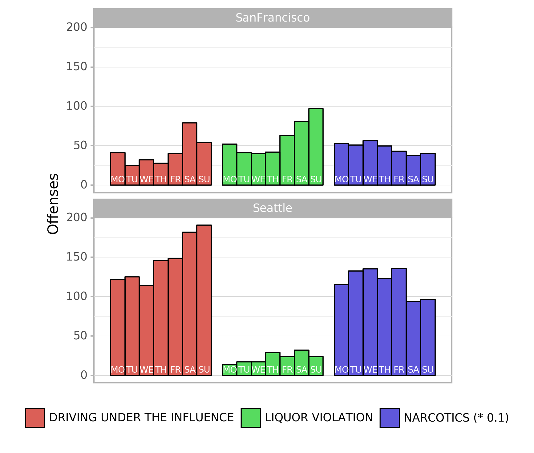
Next, the temporal occurrence of these offenses is investigated. As shown in Fig. 2 the number of recorded incidents varies over the weekdays (note that the number of narcotics incidents is scaled by a factor of 10 for visual reasons). It is obvious that alcohol related offenses are are most common at the weekends in both cities. Furthermore, narcotic reports on weekends are lower in both cities, too.
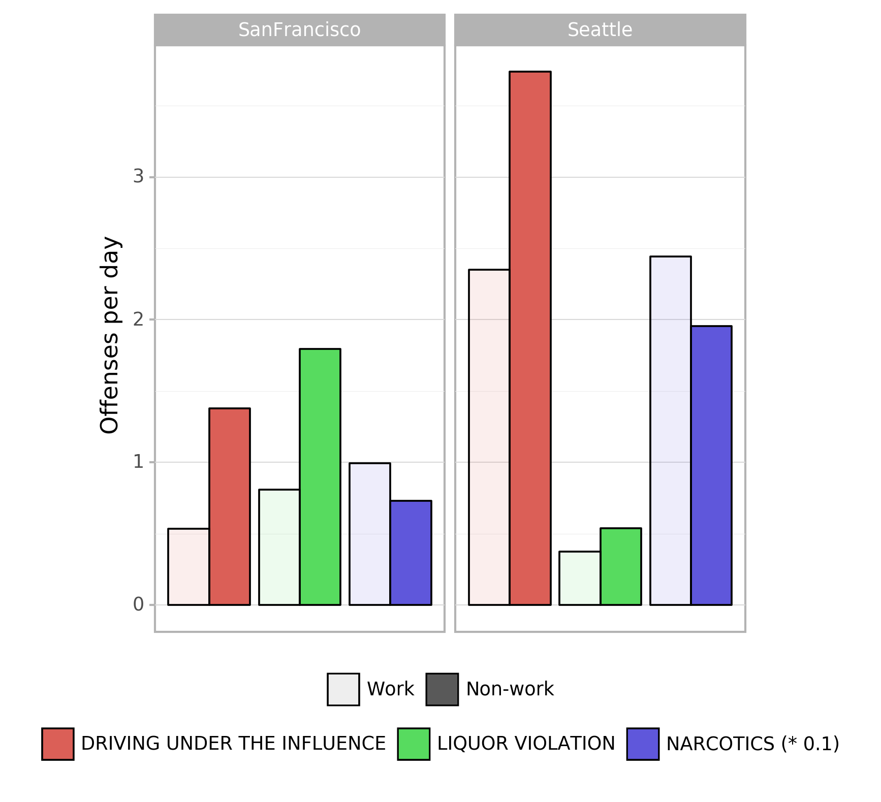
This effect can also be clearly seen in a work-day/ non-work-day plot (Fig. 3). Here, the offenses were grouped by weekdays (non-work weekend ranges from Friday after 8pm till Monday 4am, US national holidays are also considered non-work-days). The number of incidents in non-work-day episodes is clearly higher for alcohol related offenses but about 20-25% lower for narcotic related offenses).
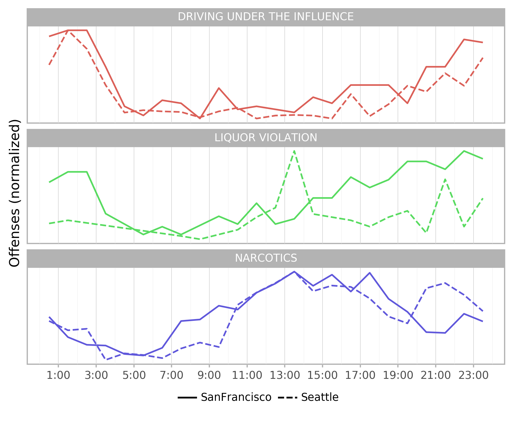
In addition to the weekly cycle, a diurnal variability of reports can be detected. In Fig. 4 the normalized number of offenses is plotted for 24-hour bins. It can be observed that “Driving under the Influence” is substantially higher from 8pm to 5am in both cities. “Liquor violation” also increased with day time (San Francisco), but the small number of incidents and the inconclusive trend for Seattle point at a schema mismatch for this class in this city. “Narcotics” incidents are dominant at daytime in both cities, with a small secondary peak from 8pm to 11pm in Seattle.
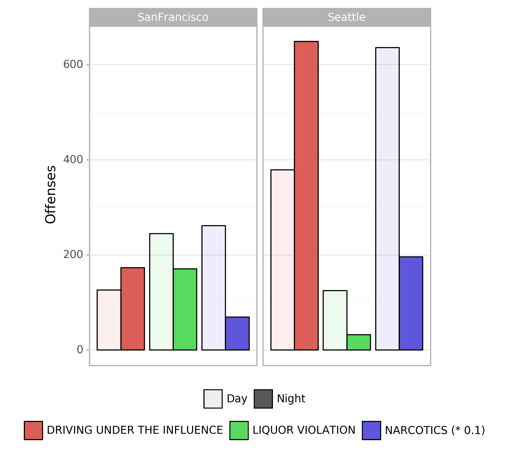
A classification in day/ night statistics (night: 9pm - 6am) further illustrates the strong difference in occurrence frequency for day and night hours (Fig. 5).
Location of crimes/ offenses
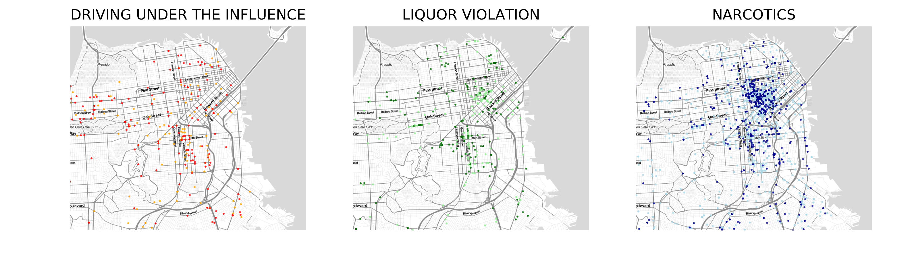
In addition to the temporal variability, the offenses also vary by their location. To illustrate this, incidents were mapped by their reported geographic coordinates.
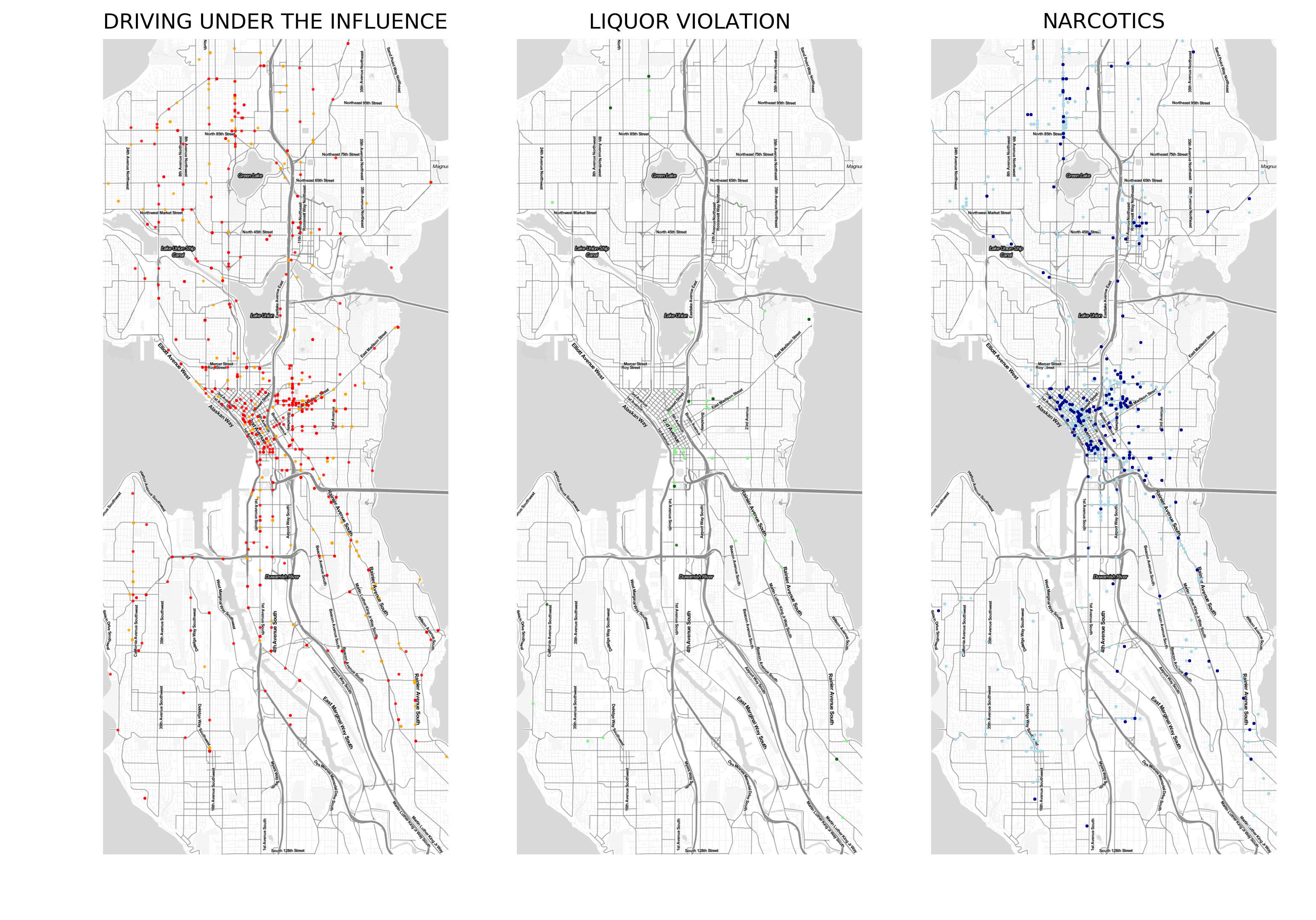
In Fig. 6 & 7 day and night incidents for the three offenses are mapped (light colors: day, darker colors: night). It is clear that “Narcotics” dominate in the CBD area of San Francisco, where as the other offenses are scattered more white spread.
In Seattle, “Driving under the Influence” and “Narcotics” dominate in the CBD and the few reported incidents of “Liquor Violation” also occur in this area, although the small sample size makes a good interpretation difficult.
Summary
It was shown that the time and location of drug and alcohol related incidents varies strongly for both San Francisco and Seattle. However, often they do follow similar patterns. A more in-depth analysis is hampered by the different data structures and a more thorough feature mapping is required for more advanced analytics.