Is this a Les Paul or is this a Strat?

I recently stumbled upon the most excellent podcast “This week in Machine Learning and Artificial Intelligence” (TWiML&AI). Sam Charrington is doing a wonderful job in presenting people and trending topics of all things AI and ML. Go check it out. It’s quality stuff!

Intro

Getting to know fast.ai

Anyways. A recent guest on his show was Rachel Thomas (Episode #138) - a university professor at the University of San Francisco and co-founder of fast.ai. To cite their company’s mission statement: “Fast.ai is dedicated to making the power of deep learning accessible to all. Deep learning is dramatically improving medicine, education, agriculture, transport and many other fields, with the greatest potential impact in the developing world. For its full potential to be met, the technology needs to be much easier to use, more reliable, and more intuitive than it is today.” (see also a blog post of them explaining why they do what they do).

So, in essence they teach state-of-the-art deep learning (DL) for the common (wo)man by providing a free MOOC on their site. What’s quite unique about it is that they decided to use a top-down approach. They basically provide almost no introduction to the basis of the field but have the students train their first deep convolutional neural network with just three lines of code and go from there… Later, they peel layer for layer and expose more and more details about the underlying fundamentals that make the machinery work. The idea is that this supposedly keeps students engaged and helps to facilitate different learning paces and styles. To make all this happen they designed a high-level wrapper that sits on top of the deep learning framework PyTorch - apparently in a similar way as Keras provides a more gentle interface to TensorFlow. As far as I understood, it was originally designed as a help for their courses but matured into a rather stable general-purpose DL library that might also be used for production…

Given that I currently teach a university course (Remote Sensing of Global Ecology (using R)) that is structured on the conventional bottom-up approach I was a intrigued about this style of teaching.

Joining the group

Sam initiated a study group shortly after the fast.ai interview. I thought I’d also check this out and so I joined to keep me motivated and here we are.

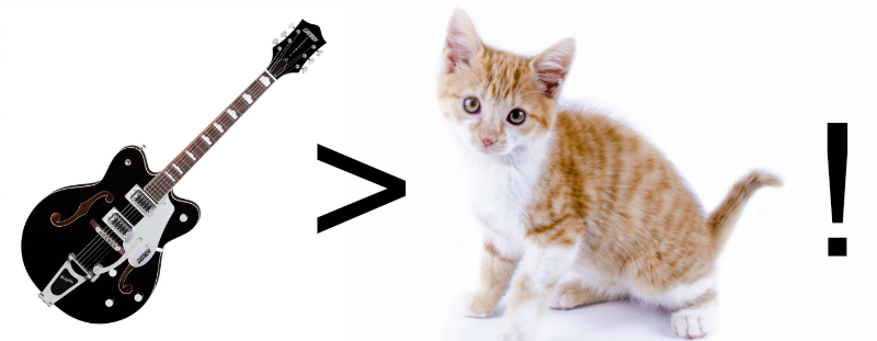
Now, in the first lesson students build the (unavoidable?) cat classifier (here it’s a cat vs. dog classifier). The whole model requires only three lines of Python code! Obviously this only works since a lot of hyper-parameters are hidden by the basic interface and a lot of choices are done by the fast.ai package by default and data is provided. Furthermore, the example uses transfer learning and thus really piggybacks on a large existing model that was trained on the massive ImageNet dataset. Nevertheless it really is quite amazing that you can get things from the ground with this little code.

The project

As an exercise students are asked to come up with their own (binary) classification problems and so I thought I’d build a guitar classifier net. To start things off I decided to go for arguably two of the most iconic electrical guitars: the Gibson (R.I.P) Les Paul and the Fender Stratocaster.

Now, a couple of things up first. While the two instruments feature very characteristic body shapes, headstocks and geometries guitars tend to come in all kinds of designs and configurations. So I’d imagine that this task is at least as challenging as differentiating between a fluffy cat and a (less so?) dog - if not much more.

Well, obviously!

Connecting to notebook server

Since I work on Macs (and none features a decent Nvidia GPU) I ssh into a GPU-equipped server that runs the jupyter notebook with GPU acceleration (it also features an anaconda installation and has the fast.ai and other required python libraries installed, I’m not discussing the setup here).

# activate the anaconda environment
source activate fastai

# start a jupyter instance 
jupyter lab --port=9000 --no-browser &

On my machine I open a ssh tunnel and bind the local port 8888 to port 9000 of the remote machine:

# connect ports
ssh -N -f -L 8888:localhost:9000 cwerner@MY_GPU_SERVER

Now I simply access the notebook via my browser at https://localhost:8888 (I also set it to be password protected).

Data setup

“First, there was data…” Well, there needs to be anyways. So one convenient way of getting hold of image data is to use Google Image Search. There is a neat Chrome extension for image harvesting - but I find that Chrome still plain sucks on a Mac so I went for another python library called google_images_download that does the same job.

# install google image downloader and pull images
pip install google_images_download

# get two batches of 1000 images (Gibson Les Pauls, Fender Stratocasters)
# I had to specify the location of chromdwriver, too
googleimagesdownload -k "gibson les paul" -pr "gibson_lp" -th -o gibson_lp -l 1000 --chromedriver /usr/local/bin/chromedriver
googleimagesdownload -k "fender stratocaster" -pr "fender_strat" -th -o fender_strat -l 1000 --chromedriver /usr/local/bin/chromedriver

For some reason the script only managed to pull ~500 images (which should still be enough for the exercise), but to get a better dataset I found that I had to manually weed through the files and delete files with missing suffixes, wrong classification, or only showing guitar parts. A neat way to do this on the Mac is simply to use the quick view in Finder and scroll through the directory and delete as necessary. I also only used the thumbnail images as the scripts currently only uses 224x224px images anyways.

Finally, I wrote some quick lines of code that created a file structure suitable for the fast.ai ImageClassifierData object.

import glob
import math
import os
import random
import shutil

# path structure: 
# guitars_small/gibson_lp/gibson_lp.1.imagedescription.jpg
gibson_files = glob.glob('guitars_small/gibson*')
fender_files = glob.glob('guitars_small/fender*')

for dir in gibson_files + fender_files:
    # create fast.ai data folder structure
    dname = os.path.basename(dir)
    npath1 = os.path.join('guitars_small', 'train', dname)
    npath2 = os.path.join('guitars_small', 'valid', dname)
    try:
		    os.makedirs(npath1, exist_ok=True)
		    os.makedirs(npath2, exist_ok=True)
    except:
        pass

    # split files into train and validation sets (80/20)   
    all_files = glob.glob(os.path.join(dir, '*.jpg'))

    idx = list(range(len(all_files))
    random.shuffle(idx)
    cut = math.ceil(0.8 * len(idx))

    train_files = [all_files[x] for x in idx[:cut]]
    valid_files = [all_files[x] for x in idx[cut:]]
		
	# copy files into appropriate folders
    for src in train_files:
        shutil.copy(src, npath1)

The model

Once the files are copied to the remote server we can create the model. First let’s import libraries and define some defaults.

import torch
from fastai.transforms import *
from fastai.conv_learner import *
from fastai.model import *
from fastai.dataset import *
from fastai.sgdr import *
from fastai.plots import *

# some constants
PATH = "data/guitars_small" # the data path
sz = 224                    # the image size 
bs = 16                     # the batch size

Now we load and fit a pre-trained model (Resnet34) to our dataset. The line containing learn.fit() executes the model training (using a learning_rate of 0.01 and for two epochs).

arch = resnet34
data = ImageClassifierData.from_paths(PATH, bs=bs, tfms=tfms_from_model(arch, sz))
learn = ConvLearner.pretrained(arch, data, precompute=True)
learn.fit(0.01, 2)

The output of the first model training using our Les Paul vs. Strat dataset

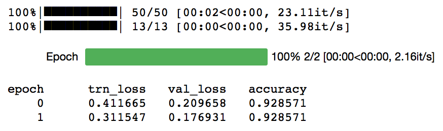
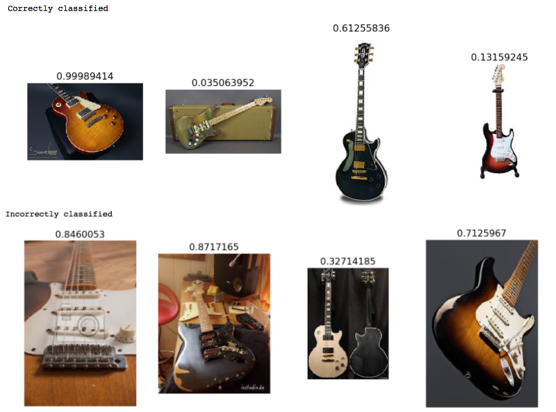
This already gives us an accuracy of 92.9%. Pretty remarkable. Now, lets see what the model identifies correctly and where it fails (I’m using some helper functions from the course for this which I do not show in this post to save space, see the GitHub repository for the full code listing; 0 = Fender Strat, 1 = Gibson Les Paul).

Some examples of correctly and incorrectly classified images

Improving the model

In essence the lesson suggests to add these improvements to get even better results:

1. data augmentation (to vary the training data by scaling, flipping and tilting images; essentially adding more labeled data)
2. fine tuning the model layers (unfreeze early layers)
3. adding learning rate annealing
4. add data augmentation at inference time

# define data augmentation (we use transforms_top_down since guitars
# could be depicted from all kins of angles (the other choice would be
# transforms_side_on)

tfms = tfms_from_model(resnet34, sz, aug_tfms=transforms_top_down, max_zoom=1.1)

# new data object with transforms
data = ImageClassifierData.from_paths(PATH, tfms=tfms)

# start the training
learn = ConvLearner.pretrained(arch, data, precompute=True)
learn.fit(1e-2, 1)

# since the model was pretrained with precimpute=True data augmentation takes no effect.
# To add this we need to switch precompute to False
learn.precompute=False

# we now add some more epochs of training (using stochastic gradient descent with restart)
learn.fit(1e-2, 3, cycle_len=1)

We now have a model where the last layer was trained while all previous layers are still frozen to the original ImageNet weights. To give the model some wiggle room to fine-tune the network to our classification domain we can unfreeze the early layers, too, and provide a separate learning rate to early, central and late layers in the model (the idea is to have small learning rates for the early layers as they should be rather generic and larger learning rates for the late layers as they characterise more specific concepts).

learn.unfreeze()

lr = np.array([1e-4, 1e-3, 1e-2])

learn.fit(lr, 3, cycle_len=1, cycle_mult=2)

Test Time Augmentation (TTA) was something I never heard about but apparently it can further improve results quite a bit. TTA computes 4 augmented test images and judges the quality at test time based on the majority vote on all five images which helps the model to generalise better.

log_preds,y = learn.TTA()
probs = np.mean(np.exp(log_preds),0)
accuracy_np(probs, y)

In my setup this final model now achieves an accuracy of 95.4%. Given the diverse input data and relatively small sample set I find that quite amazing.

Some evaluation

First, let’s look at the confusion matrix. This illustrates the accuracy of the model for the individual classes (the diagonal is the correct prediction for all classes). In total there were 102 Strat and 94 Les Paul images in the validation dataset (the split was 80/20 of the total images).

Confusion matrix of model predictions

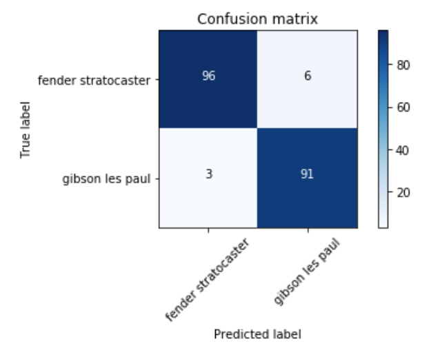
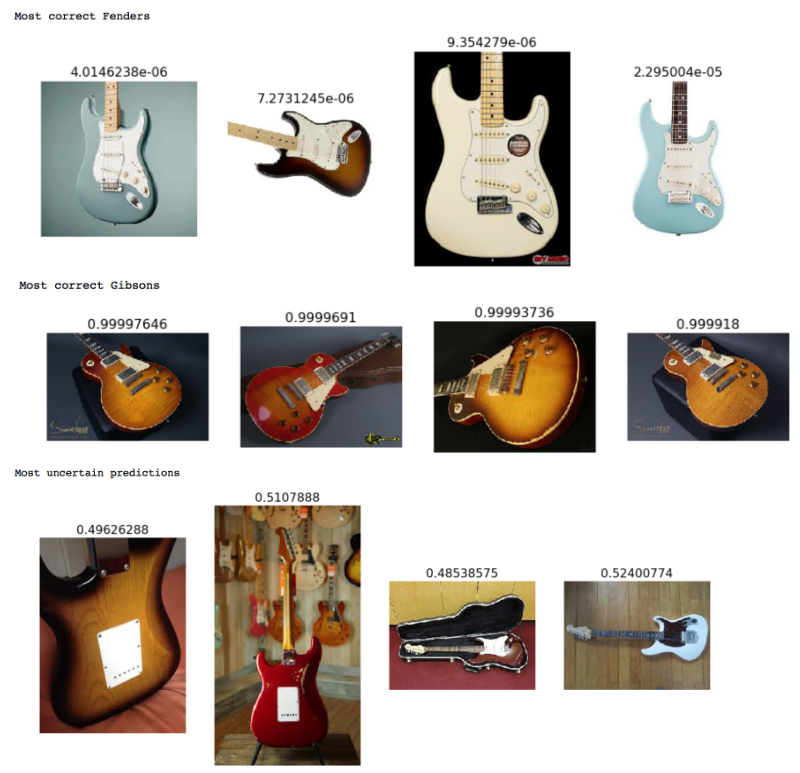
As we can see the model incorrectly predicted three Les Pauls to be Strats and six Strats for Les Pauls. Now let’s look again at some images (top: most confident Fenders, middle: most confident Gibsons, bottom: most uncertain images)

Best classification results and results where the model is most uncertain about the class.

Next steps

Now, while the results are not as great as the dog vs. cat classifier in the fast.ai lesson that consisted of a much larger dataset, I still believe results are quite neat. I currently think about the following steps for further experiments:

1. Get more images: the number of images is still small (400 training, 100 validation images per class)
2. Try the same exercise with the full resolution images (I have the feeling that the thumbnails are too small for the network and sz setting
3. Further selection of images that are a) too small, b) have multiple guitars in the image, show too little of the guitar (some only had the fingerboard or the headstock), c) remove images with backside shots.
4. I also want to extend this to mulit-class classification: Gibson Les Paul, SG, Firebird, Explorer and Fender Stratocaster, Jaguar, Mustang and Telecaster. This should be interesting!